Pile Under Lateral Load According to the EC2 General Method

General Eurocode 2 Method Applied to Concrete Piles: Managing Second-Order Effects, Stresses, and Displacements

This article presents a nonlinear EC2-type approach (§5.7) for the design of a single pile under lateral loads.

The analysis of an isolated pile under lateral load is a common use case, usually treated as elastoplastic on the soil side and linear elastic on the pile side. The subject can also be seen as the analysis of a slender reinforced concrete column with intermediate elastic supports.

Once the soil behaviour and, in particular, the plastification depth are determined, this approach allows for an accurate assessment of second‑order effects, SLS and ULS stress criteria, and deformations, relying on the full EC2 framework.

Introduction to the Example

 

Typical Calculation Steps for a Pile Under Lateral Load

 

To perform the calculation of a pile under transverse loading, foundation engineering offices usually proceed in two steps:

The first step consists of the structural analysis of the entire pile+soil system at ULS, using the following assumptions:

• the reinforced concrete pile is assumed to be linear elastic (EC2 §5.4 approach)
• the lateral reaction of the soil is evaluated in each layer according to EC7, and in France in particular using NF P94‑262 Annex I. This reaction is bilinear, elastic–plastic.

The structural analysis provides the internal forces M,N to be considered in the pile.

The second step then consists of performing the section design itself, generally at the location of the various critical sections (maximum moment, reinforcement cut‑offs…), in the form of checks based on successive tests of longitudinal reinforcement sections.

This step is carried out through the construction of M–N interaction diagrams depending on the reinforcement ratio of the tested pile.

 

Approach Proposed in This Article

 

In this article, we propose a different approach to the analysis of a pile subjected to a lateral load, using the general method of Eurocode 2.

This study focuses on accurately modelling reinforced concrete behaviour to allow:

• the regulatory assessment of second‑order effects in the pile at ULS
• the optimisation of the reinforcement cage
• the evaluation of stresses and displacements at the pile head at SLS

The lateral reaction and the bearing effect from shaft friction are modelled using lateral springs or discrete forces regularly positioned along the pile, and are calculated based on pressiometric soil assumptions according to NF P94‑262.

 

 

Context of the Example

 

Project Description

We consider a reinforced concrete building founded on 40 piles, including a semi‑buried substructure subjected to a permanent asymmetric earth pressure. The entire horizontal load on the building is transferred to the ground through the piles, via the 18‑cm thick ground slab acting as a horizontal diaphragm.

The suspended slab acts continuously over grade beams arranged perpendicular to the earth pressure.

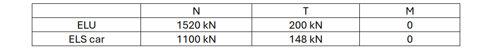
We focus on the design of a typical pile, for which the structural analysis performed by the design office provides the following actions to be considered at the pile head:

The soil consists of silts with the following pressiometric characteristics: Em = 8 MPa, pl* = 0.8 MPa, pf* = 0.5 MPa.

The piles are bored using a continuous flight auger with parameter recording and enhanced quality control, and are constructed with C30/37 XC2 concrete, 52 cm diameter, and 6 HA16 reinforcement.

The steel reinforcement has characteristics f_yk = 500 MPa, class B, and is provided with 7 cm cover (concrete cast directly against earth, EC2 §4.4.1.3(4)). We consider u = 10 cm (distance between surface and bar axis).

The piles are executed after excavation of the substructure, with positioning and inclination tolerances of e₀ = 10 cm and ϑ₀ = 0.02 cm/m, according to the execution standard.

However, since no specific information was provided in the contract documents regarding the consideration of execution tolerances, these effects are assumed to be included in the load transfer provided by the design office. (For more on execution tolerances and interfaces between design offices, see: Load transfer on piles, construction tolerances, and support stiffnesses)

 

Objectives of the Study

 

In our example, we aim to verify the following:

• [1] check the pile resistance at ULS, considering possible second‑order effects
• [2] verify the compressive stress in the concrete at SLS (quasi‑permanent)

 

Calculation Assumptions

 

Concrete and Soil Creep Assumptions

 

The loads acting on our system are mostly long‑term actions. The SLS load on such a building contains at most about 20% variable loads, while the asymmetric earth pressure is a permanent action.

For evaluating concrete and soil creep, we simplify by considering that all actions are long‑term (including variable loads).

For concrete, NF P94‑262 allows a long‑term modulus of E_cm/3 (§6.4.1 (12)), which corresponds to φ_inf = 2.

For the soil, NF P94‑262 does not modify shaft friction depending on load duration. For lateral reaction, it provides a short‑term elastic‑plastic law and proposes dividing the elastic stiffness by 2 to obtain the long‑term law, while keeping the plastic value unchanged (§I.1.4).

We therefore adopt:

• For SLS QP and SLS long‑term:
  • concrete modulus 0.33 E_cm, i.e. φ_ef = 2
  • lateral reaction: 0.5 K_i

• For ULS:
  • concrete modulus 0.4 E_cm, i.e. φ_ef = 1.5
  • lateral reaction 0.57 K_i

Note: see also this article on creep coefficient evaluation at ULS.

 

Soil Assumptions: Lateral and Axial Reactions on the Pile

 

The determination of lateral and axial reactions along the pile is straightforward and follows NF P94‑262.

For axial friction, we assume full mobilisation of shaft friction for each limit state considered.

For the lateral reaction, we use an elastic‑plastic reaction law, modified by a creep coefficient and by a reduction near the ground surface.

 

A Pre‑Processing Spreadsheet

 

As the MGI tool is generic, a dedicated pre‑processing spreadsheet prepares the required input data. It acts as the interface between:

• soil layers and their pressiometric parameters
• pile characteristics (diameter, type)
• pile head loads

and the input data required for the actual pile calculation:

• boundary conditions and intermediate elastic supports along the pile
• discrete loads along the pile

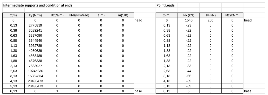
By convention, the x‑axis follows the pile axis downward from x = 0 (head) to x = 6.13 m (base). The mesh is refined near the pile head (25 cm spacing) and coarser in depth (1 m spacing).

The boundary conditions table includes:

• Kx = “1” at x = 6 m. “1” means infinite stiffness, representing axial restraint at x = 6 m.
• Ky represents the discretised lateral stiffness
• kMz represents any rotational stiffnesses (here = 0)
• a and m represent, where applicable, support width and monolithicity. In this example, these notions are irrelevant, so we keep default values a = 0 (point supports) and m = 0 (non‑monolithic support).

The discrete load table includes:

• the pile head loads
• the “bearing” effect from axial friction Nx along the pile

 

Implementation of Soil Plastification

 

In this initial version of the spreadsheet, the soil is assumed to be elastic over the full depth, i.e. plastification depth is zero.

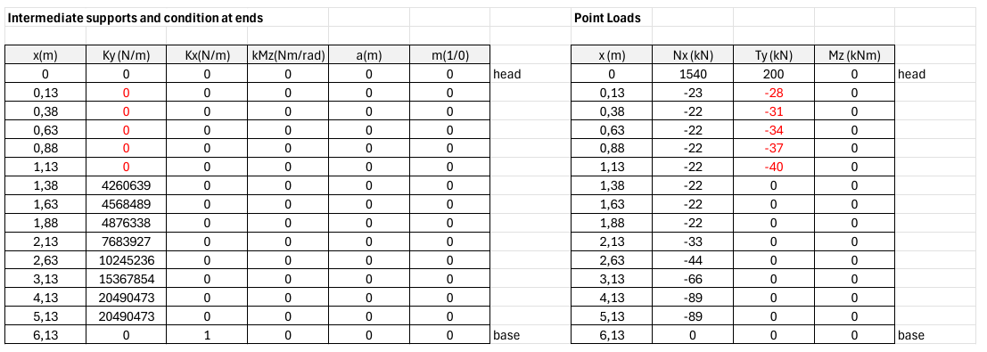
After a first simulation, the computed soil reactions (at x = 0.25 m, x = 0.75 m, x = 1.25 m) are compared to the corresponding plastic values r1. This gives the depth over which the soil should be considered plasticised.

The tables are updated accordingly and the calculation is rerun. One or two iterations are generally sufficient to obtain the final soil model.

For example, below, the plastification depth has been updated to 1.20 m. The pre‑processing spreadsheet has removed the first “springs” and replaced them with stabilising horizontal forces (in red).

The spreadsheet is available for download here (OpenLAB registered users):

 

Assumptions for the Concrete of the Pile

 

The concrete of the pile is C30/37, exposure class XC2, and the pile is constructed using a continuous flight auger with parameter recording and enhanced quality control. In accordance with NF P 94‑262 §6.4.1, we therefore adopt f_ck^* = 21.2 MPa, giving:

• at ULS: f_cd = 16.9 MPa
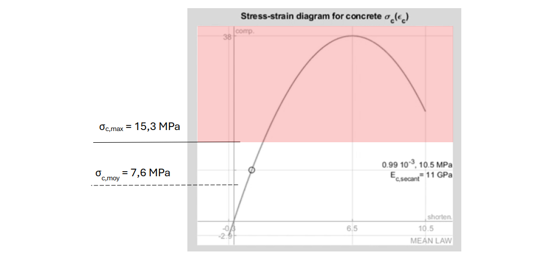
• at SLS (characteristic): σ_c,moy = 7.6 MPa and σ_c,max = 15.3 MPa

 

 

Using the MGI Tool

 

Sequence 1: Data Input and Soil Model Adjustment

 

Initialising the Simulation

 

The following video illustrates the model setup, including:

• importing the elastic supports along the pile from the pre‑processing spreadsheet
• resetting the construction camber (no geometric imperfection)
• importing the loads along the pile from the pre‑processing spreadsheet
• setting the concrete strength f_ck = 30 MPa and creep coefficient φ = 1.5
• defining the 52 cm circular formwork
• defining the reinforcement of 6 HA16 bars placed around the perimeter at 10 cm cover

This initial set of assumptions considers the soil to be elastic over the entire depth.

 

Adjusting the Plastification Depth

 

The first simulation yields elastic lateral reactions of 48, 45 and 40 kN for the first three springs down to 0.63 m, whereas their respective plastification thresholds are 28, 31 and 34 kN.

The soil plastification depth must therefore be taken into account.

A plastification depth of 1.20 m is tested for the second simulation. This value, higher than 0.63 m, anticipates the fact that plastification near the surface increases the loads and will likely plastify additional springs.

The second simulation gives elastic lateral reactions of 42, 30 and 22 kN for the first elastic springs located between 1.38 m and 1.88 m, while their plastification thresholds are 43, 46 and 50 kN.

We conclude the validity of the soil model and proceed to the pile design sequence.

 

Sequence 2: ULS Design

 

Switching to the “Local Structural Analysis and Design of Sections” tab allows examination of the stresses in the “exact” solution at all pile sections, particularly in the critical one.

 

Concrete Behaviour in the Pile and ULS Criterion

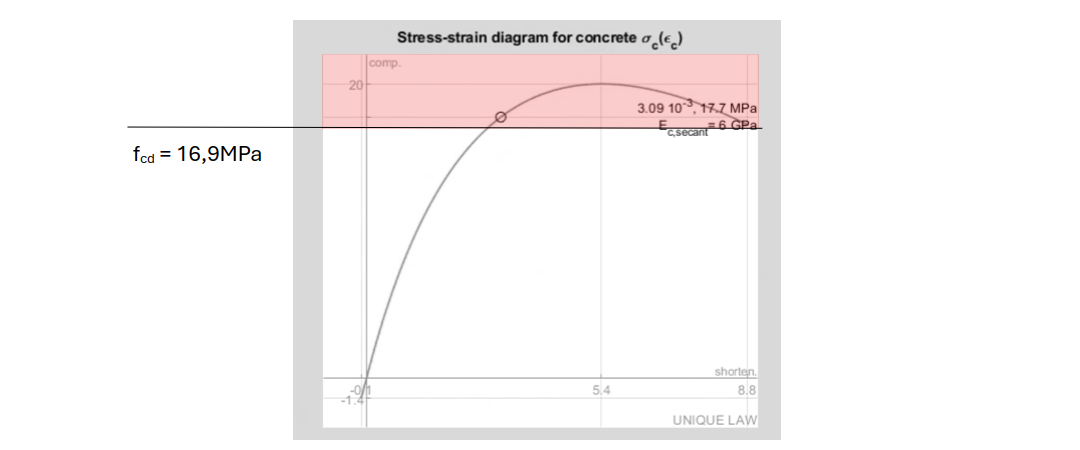
The ultimate allowable stress for compressed concrete is f_cd = 16.9 MPa, calculated using formula (6.4.1.2). This value depends on f_ck* = 21.2 MPa and not f_ck = 30 MPa.

NF P94‑262 also specifies that f_ck* should be used “only for the limit states of concrete in compression” (§6.4.1(10) NOTE 1), and the CEREMA application guide (available here) explicitly states that E_cm must be computed from f_ck, not f_ck*.

Accordingly, the concrete behaviour law used in our calculation is calibrated with f_ck, not f_ck*. More precisely, the initial modulus is not E_cm, but 1/(1+φ) · E_cm / γ_CE, and the curve follows the EC2 general stress–strain model, not the parabolic‑rectangular one.

 

Reinforcement Strengthening

 

In our simulation, the “ULS concrete compression” criterion is not satisfied at the critical section: 17.7 MPa > 16.9 MPa.

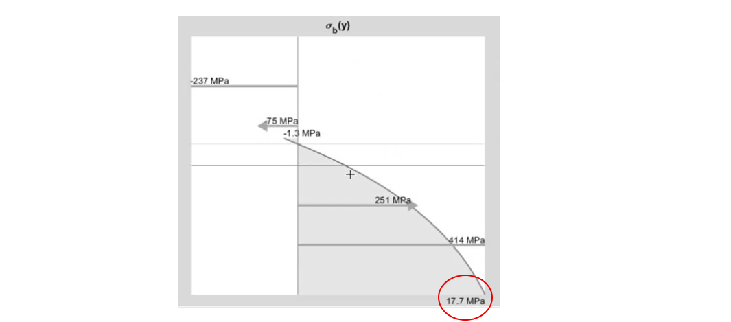
To decrease the stress in this highly loaded region, the reinforcement is increased by doubling the 6 HA16 bars with 6 HA14 bars over a height of 2 m. In the settings, dx_end = –4 m stops the added bars 4 m before the end of the segment (i.e. at depth 2.13 m).

The new structural analysis is slightly more favourable because the pile stiffness has increased, and the ULS concrete compression criterion is now satisfied at the critical section (x = 1.63 m) and just after the bar cutoff at x = 2.13 m.

Note: Since the tool does not handle anchorage, execution drawings must specify L = 2.13 m + L_bd for the 6 HA14 bars.

 

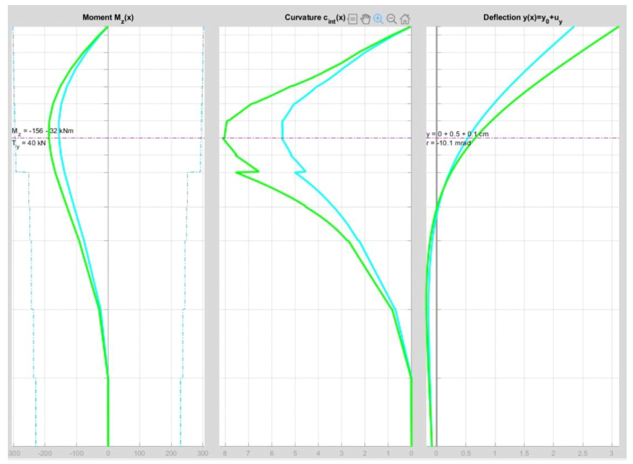
Second‑Order Effects

 

The structural analysis includes second‑order effects, which can be visualised by superimposing the curves without second order (blue) and with second order (green).

In this example, the effect is significant: the moment in the critical section increases by 32/156 = 20%.

These curves also highlight the impact of cracking on the inertia in the critical zone, where curvature increases faster than moment. A local drop in inertia is also visible beyond the cut‑off of the 6 HA14 (bend in curvature).

Compared with usual methods, the general method applied along the entire pile provides the “exact” EC2‑consistent structural analysis:

• without approximation of the pile inertia
• without assumptions on the deflected shape
• ensuring deformation compatibility — not guaranteed with interaction diagrams

 

 

Sequence 3: SLS Stress Checks

 

Updating the Model for SLS (Characteristic)

 

The SLS calculation requires updating the pre‑processing, particularly:

• updating pile head loads (SLS values)
• updating the axial friction resistance
• updating the lateral reaction coefficient Kv/Ki = 0.5
• resetting elastic supports (plastification depth reset to zero)

The pile model is then updated:

• updating boundary conditions and intermediate supports
• selecting “SLS” as the analysis type
• updating loads along the pile from the pre‑processing spreadsheet
• updating the creep coefficient φ = 2

Selecting SLS switches the concrete material laws to mean values rather than design values.

As before, the first simulation shows plastification of the first spring only. The plastification depth is adjusted to 0.30 m and the second simulation provides a valid soil model.

 

SLS Stress Verification

 

The concrete behaviour law for SLS is built the same way as for ULS, based on f_ck and not f_ck*.

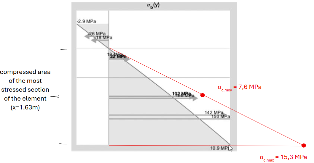
The SLS concrete compression criterion requires checking σ_c,max and σ_c,moy in the compressed zone of the most loaded section (§6.4.1(9) NOTE 1), which amounts to positioning the following “template” on the stress block at x = 1.63 m:

Note: the graphical display of steel stresses is difficult to read due to the proximity of HA16 and HA14 bars; zooming helps.

This template must also be applied to the section right after the 6 HA14 cutoff:

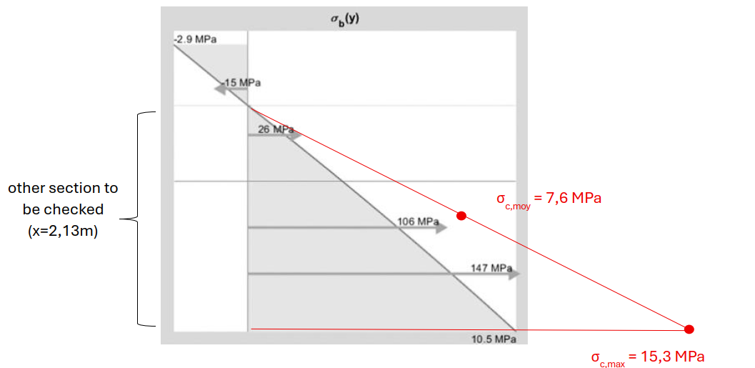
Both stress diagrams remain within the template: the SLS compression criterion is satisfied.

The tool can similarly check other EC2 criteria: crack width, steel stress limitation, pile deformation.

 

Role of Reinforcement in Meeting f_cd, σ_c,moy, and σ_c,max

 

In our example of a laterally loaded pile—and in general—pile reinforcement plays a major role in the compression resistance of reinforced concrete sections. Strengthening the reinforcement at the pile head can easily reduce σ_c,ULS enough to satisfy f_cd and avoid increasing the pile diameter. For a 20‑m pile, 20 kg of steel can save 4.5 tons of concrete.

The same applies at SLS.

Although σ_c,moy and σ_c,max (§6.4.1(9)) are sometimes interpreted as checks to be done ignoring reinforcement, the CEREMA guide (available here) clarifies that reinforcement must indeed be considered (example 4 of the guide).

Assume a concentrically loaded pile with reinforcement ratio x%. The allowable SLS characteristic stress can be expressed from σ_c,moy as:

Assuming C25/30 concrete and a typical 80% permanent load ratio (E_c,ef = 1.14·10^? Pa):

The effect of reinforcement on the SLS allowable stress is far from negligible:

Depending on the configuration, reinforcing a few piles can be a cost‑effective strategy to avoid changing the auger diameter, considering that increasing pile diameter greatly increases concrete volume: +122% for large piles (920 mm) and up to +153% for small piles (420 mm).

Where positive shaft friction is significant in the upper layers, reinforcing only the pile head down to the depth where the extra steel load is compensated by shaft friction can also allow reducing the diameter of all piles.

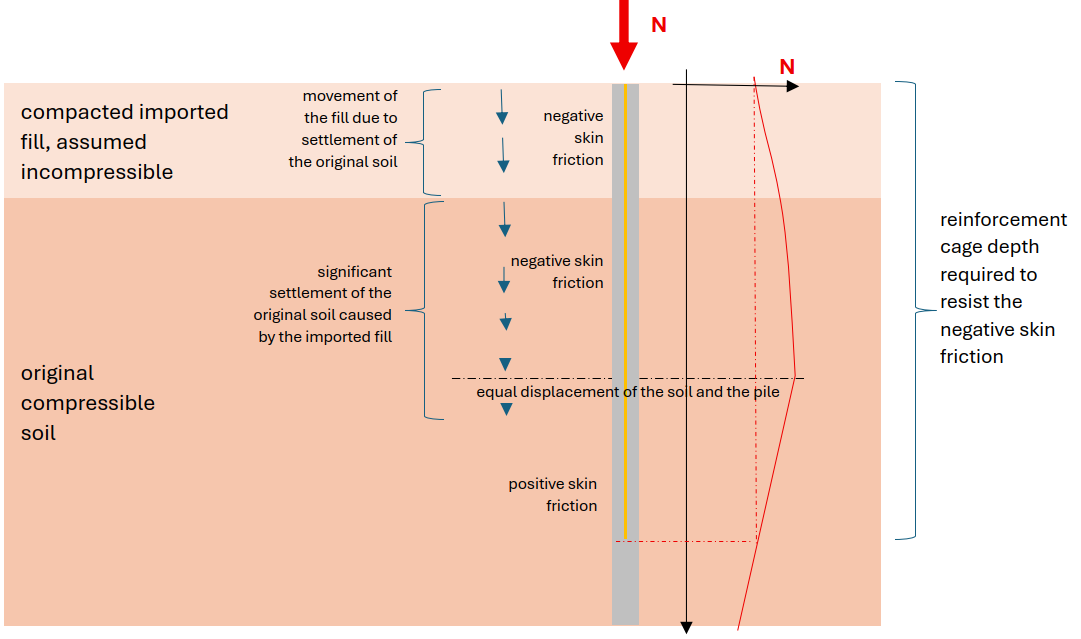
Conversely, in the presence of negative skin friction, reinforcing piles allows absorbing the increased axial force—provided the reinforcement extends deep enough into the layers with positive friction.

 

Conclusion of the Example

 

The design of a pile under lateral load is a valid use case for the “integral general method” tool, leveraging the full EC2 framework for sizing and optimising a pile, provided that a pre‑processing spreadsheet is created to facilitate iterations.

This spreadsheet enables application of the regulatory reaction of a single‑layer or multi‑layer soil, here for a pile loaded at its head, but it can also be adapted to other configurations such as group effects or g(z).

Once the soil model is validated, the tool can compute the exact solution based on the engineer’s design choices—lengths, bar sizes, concrete properties—without any assumptions about modulus, inertia, cracking, deformation shape, or transfer length.

Furthermore, the calculation directly applies the Eurocode 2 material constitutive laws to determine stresses in the materials as well as displacements at the ULS and SLS, which removes the need for interaction diagrams.

It is commonly assumed that piles embedded in the ground are unlikely to buckle, which is true, but this does not mean that second‑order effects can be disregarded. These effects can indeed amplify the design forces at the ULS and lead to exceeding the stress criteria defined at the ULS, as observed in our example. It may therefore be relevant to consider these effects in the design of piles. 

In a future example, we will see that the tool can also handle, for instance, columns of arbitrary section embedded in piles, subjected to various support conditions and loading scenarios.