Design of a Mast Using the EC2 General Method – Configuration and Optimisation

The partially fixed mast is a common configuration of reinforced concrete structures, which nevertheless remains poorly documented in the literature. Yet a partial fixity is a delicate assumption to handle.

This example offers a review of the data input process and the justification of such a calculation, according to the general EC2 method reduced to one critical section (MG1). It especially details various reminders and points of attention to monitor in order to successfully perform the design.

The end of the example shows the exact solution to the problem and the possible optimisation made possible by the integral general method (IGM).

 

 

Note: This example completes the more general dossier dedicated to the “General Method of EC2 and Usage Limitations”. The reader may also refer to it for the theoretical part.

 

Presentation of the case

 

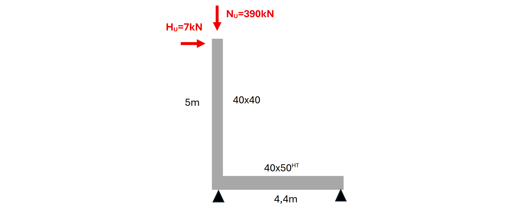
In this example, we consider a simple mast whose section properties are constant along its axis and correspond to the following diagram:

 

 

We assume additionally that the mast is restrained out of plane, and that the geometric imperfection (verticality or positioning tolerance) is included within the horizontal force H_u shown below.

Lastly, we assume a concrete creep coefficient under ULS loading of φ = 1.

For the grade beam, the following additional assumptions are made:

• the grade beam is subjected to no load other than that transferred from the column
• the grade beam uses the same materials as the column

Note: if the grade beam were subjected to gravity loads, a verticality defect in the column would need to be considered, imposed by the rotation at the support of the grade beam.

The study of this project is therefore equivalent to the study of a column free at the top and partially fixed at the base, which we analyse using the general EC2 method, or more precisely its simplified option reduced to the study of a single critical section (MG1).

 

First step: determining the rotational stiffness exerted by the grade beam on the column base.

 

We assume here that the grade beam remains within its elastic domain under the ULS loading that governs the column design. We can therefore use the usual formulas from strength of materials:

k_beam->column = 3 E I / L

E: Since we are in the context of second-order column analysis, we use the design behaviour law, including creep. Hence: E = E_cm/γ_CE / (1+φ) = 1.3×10¹⁰ Pa.

I: We must also adopt a conservative inertia for the grade beam, to remain on the safe side for the column design. Since the grade beam is in simple bending, we assume its cracked inertia equal to 1/2.5 of its uncracked formwork inertia.

I = (0.4×0.5³/12) / 2.5 = 1.7×10^-3 m⁴

L = 4.40 m

We therefore obtain: k_beam->column = 3 E I / L = 1.5×10⁷ Nm/rad.

 

Second step: determining the buckling length of the column

 

Knowing the stiffness k_beam->column allows us to determine the flexibility at the lower end of the column model:

s₁ = 1/k_beam->column · E·I/L

To remain on the safe side, we now consider:

• a higher E, e.g. E_column = 1.3×10¹⁰
• a higher I, as the column under bending–compression is likely to be uncracked under the governing load combination: I_column = (0.4×0.4³/12) = 2.1×10^-3 m⁴

This gives: s_inf,column = 0.36.

Since the column is free at the top, its upper end flexibility is infinite: s₂ = +∞

With the column unbraced at the top, we use formula (5.16) of EC2, taking the limit of l₀ as s₂ tends to infinity. Using the notations of this example:

i.e. L_f = 2.52 L, so L_f = 12.6 m.

The future EC2 proposes a different formula (O.10). Applying it gives:

i.e. L_f = 2.73 L, or L_f = 13.65 m.

Note: For the continuation of the example, we adopt the result of the future EC2 formula.

 

Third step: determining the equilibrium point of the critical section

 

The MG1 method is most often implemented in the form of a spreadsheet.

This covers the case of straight columns with constant section and bi-symmetric reinforcement, for three common formwork shapes: rectangular, circular, and diagonal.

Remark: The “diagonal” case may seem redundant with the rectangular case, but for square columns and depending on reinforcement ratios, buckling along the diagonal may occur before buckling around principal axes.

 

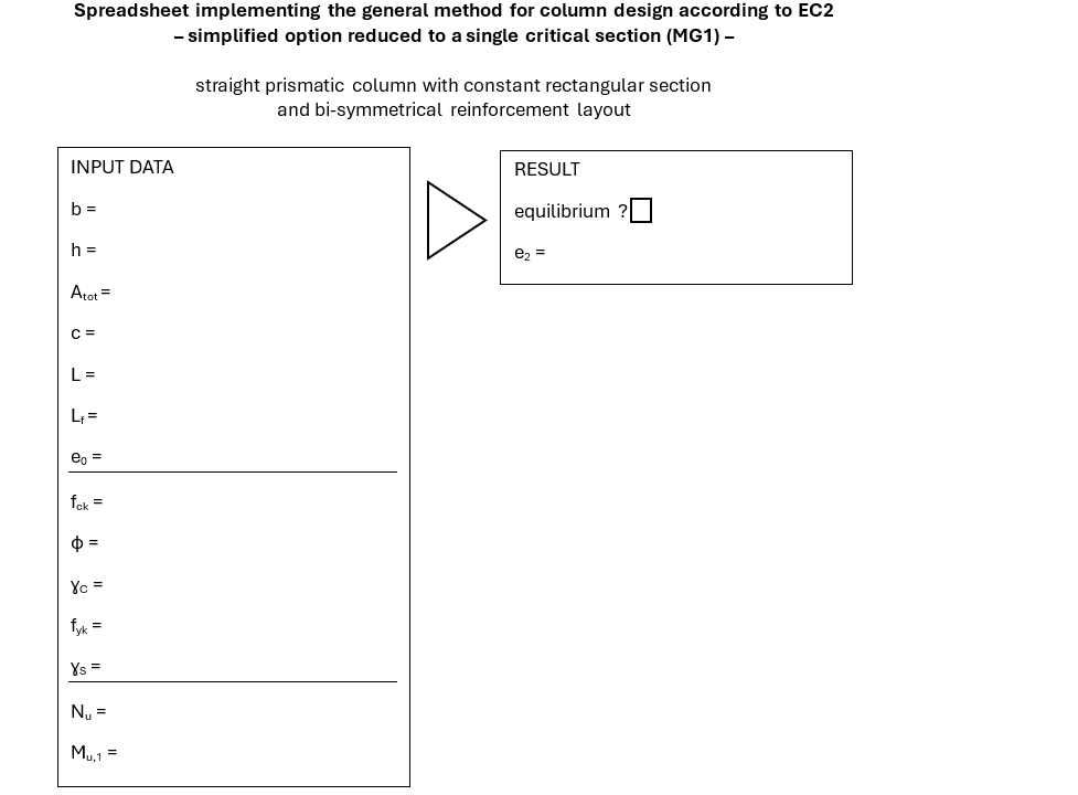
The spreadsheet determines the stable equilibrium point—if it exists—between the “internal” curvature of the RC section and the external curvature given by the structural model (RDM), at the critical section of the equivalent mast assumed to deform sinusoidally.

The main added value is the determination of the second‑order additional eccentricity e₂, obtained iteratively.

Recall that in MG1, the critical section is the section of perfect fixity of the equivalent mast of height L_f/2, which must not be confused with the partial fixity section of the real column.

Points of attention when completing the spreadsheet:

• The first‑order moment to be entered is that of the critical section: M₁ = H_u × L_f/2 = 48 kNm (and not H_u × L/2).

• Check the meaning of A_tot in the spreadsheet. In the rectangular sheet, A_tot usually means the total steel area in the top and bottom fibres. Here: 6HA16 = 12 cm² (not 8HA16).

• The additional eccentricity is sometimes automatically accounted for from the effective length, but here it is set to 0 since it is included in H_u.

Once these steps are done, the spreadsheet can be completed and the solution obtained:

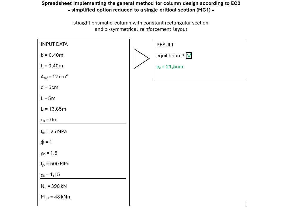
The equilibrium point is found; the critical section is verified.

The verification can stop here for the ULS normal force check of the entire column, since convergence to the equilibrium point mechanically justifies the fixity section of the real mast.

No bar terminations or formwork reductions are needed along the height, even though the moment decreases towards zero at the top, because the constant‑section assumption is inherent to MG1.

Note that we justified a fictitious section to deduce the validity of all real sections. However, none of the real sections experiences the perfect‑fixity moment of the equivalent model—this paradox is inherent to MG1.

 

Fourth step: determining the fixity moment and verifying the grade beam

 

Once the column is verified, second‑order effects must be transferred to the supports and included in their design.

Here, we must determine the moment at the real base connection between the column and the grade beam, then design the grade beam, and ideally check whether the assumed inertia of the beam is indeed a lower bound.

From the obtained value of e₂, the external eccentricity along the entire column can be determined.

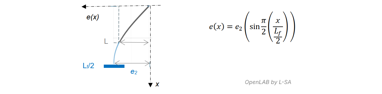
In particular, at the real fixity (x = L):

We can then verify the grade beam and check whether I_beam ≥ I_nf / 2.5 to validate our initial assumption.

By performing a new column simulation with N_u = 400 kN, equilibrium is no longer achieved: N_u = 390 kN is the ultimate critical load according to MG1.

 

Digression on the partial fixity stiffness

 

According to MG1, the rotation at the real column base can be obtained by differentiating the previous formula:

We can then verify whether k = M/ϑ.

 

Here we obtain 5.6×10⁶ Nm/rad and observe that this does not match the target rotational stiffness of 1.5×10⁷ Nm/rad assumed initially.

In reality, the sinusoidal deformation assumption leads to the more general relation between the base stiffness of a mast of length x with partial fixity and its buckling length:

The obtained stiffness depends not only on the buckling length but also—unavoidably—on the applied loads. Yet formulas 5.16 (current EC2) and O.10 (future EC2) include no such load dependence.

This discrepancy is inherent to MG1 and places us safely on the conservative side.

 

The exact solution to the problem

 

The integral general method gives the exact solution through a simpler, more accurate, and more easily verifiable approach.

The following video, commented below, shows the model input and the exact calculation results.

Model configuration

 

• Support conditions:
  • top support at x=0, bottom support at x=5 m
  • removal of lateral stiffness Ky at the top (free end)
  • removal of “support widths” a: in this isostatic column study, moment capping at supports is not applied
  • addition of partial rotational stiffness at the base: K_M = 1.5e7 Nm/rad

• no initial lateral imperfection (assumed included in H_u)

• Loading configuration:
  • normal force N_z = 390 kN at x=0
  • lateral force T_y = 7 kN at x=0

• Material configuration:
  • neglecting concrete tensile strength: f_ct = 0 MPa
  • including creep: φ = 1

• Formwork: rectangular section 40×40

• Reinforcement: 8 HA16 around the perimeter

The solution

 

The calculation converges to equilibrium: “2^nd ORDER COMPLETED”.

• The “Global Structural Analysis” tab shows graphical results for moment, curvature, and total deflection along the column, including second‑order effects. The curvature is not sinusoidal and presents an inflection point at the cracking moment.
• The “Local Structural Analysis and Design of Sections” tab provides local diagrams of the internal behaviour of the column.
• The column diagram shows support reactions including second‑order effects (M_z = 47 kNm).

The curvatures shown in the third tab match those in the second tab. All results can be verified graphically step by step.

For this case, both concrete and steel are lightly stressed, with maximum stresses not exceeding 100 MPa (steel) and 6 MPa (concrete).

Optimisation of the design

 

The IGM tool allows optimisation of the structure. The following video, commented below, shows the optimisation in three steps.

Formwork optimisation

 

• change formwork from 40×40 to 30×30
• calculation does not converge: “BUCKLING”
• change formwork to 35×35
• calculation converges; base moment increases from 47 kNm to 56 kNm

Reinforcement optimisation

 

• a second segment is created at x = 2.50 m to reduce reinforcement in the upper part: from x=0 to x=2.50 m, reinforcement is halved to 4 HA16 (A/B = 0.65% OK)
• calculation converges; reinforcement reduction has no significant effect on the second‑order moment (still 56 kNm)
• the upper segment is extended to x = 4.50 m
• calculation converges again, second‑order moment becomes 60 kNm

Important remark: The IGM model allows varying the section along the element in constant‑section segments. The method assumes all sections are fully effective in concrete and steel; execution drawings must therefore include sufficient anchorage lengths and additional concrete cover where necessary.

Using the integral general method allowed in this example:

• a 25% reduction in concrete volume
• a 45% reduction in longitudinal reinforcement

 

See also, on this topic, the broader introductory article presenting the advantages of a integral general method for Eurocode 2 : An Integral General Method (IGM) in accordance with Eurocode 2

We hope this article has been helpful. Feel free to share your suggestions for improvements or corrections in the article comments available at the bottom of this content (OpenLAB members only).